Conditional Formatting... Simple Tools.. Helpful Results

Today we will share with you some tips on how to use Excel's Conditional Formatting. This tool is very useful when you want to find specific information from a LOOONG List of stuff!

It is really quick and easy. the first step is to highlight what do you want to search. Example: I have a list of staff and the number of sales this month:

And i want to find which staff has reached this months target, lets say that the target is 300.

STEP 1: Select the data: Just simply select the data (in this case the sales column)

STEP 2: Go to Home, then select "Conditional Formatting":

This time i want to use "Highlight Cell Rules" to find which staff has more than 300 sales.

STEP 3: Choose "Greater Than":

STEP 4: A box will pop up, insert the value (which is 300 for this example):

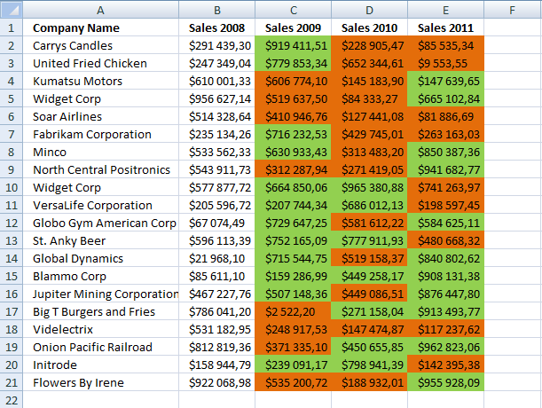
Then choose any color that meets your taste, then click OK. As a result you will see:

Here we can see staff number 6, 13 and 18 has reached the target!

There are many other things you can do with conditional formatting, you just have to simply explore!

Here is a short list on what other functions it has:

1. LESS THAN: Highlights Cells that are less than X
2. BETWEEN: Highlights Cells that are between X and Y
3. EQUAL: Highlights Cells that are equal to X
4. TEXT THAT CONTAINS: Highlights cells that has a specified letter, word, or a sentence.

Theres many more! you can even try the top/bottom rules aswell.

Have fun! I hope this is useful.

Want to learn more about Excel, SPSS or Statistical Analysis? Contact us today!